Your continued donations keep Wikipedia running!

Exogenous growth model

From Wikipedia, the free encyclopedia

The Exogenous growth model, also known as the Neo-classical model or Solow growth model is a term used to sum up the contributions of various authors to a model of long-run economic growth within the framework of neoclassical economics.

[edit] Development of the model

The Neo-classical model was an extension to the Harrod-Domar model that included a new term, productivity growth. The most important contribution was probably the work done by Robert Solow; in 1956, Solow and T.W. Swan developed a relatively simple growth model which fit available data on US economic growth with some success^[1]. Solow received the 1987 Nobel Prize in Economics for his work on the model.

[edit] Extension to the Harrod-Domar model

Solow extended the Harrod-Domar model by:

Adding labor as a factor of production;
Requiring diminishing returns to labor and capital separately, and constant returns to scale for both factors combined;
Introducing a time-varying technology variable distinct from capital and labor.

The capital-output and capital-labor ratios are not fixed as they are in the Harrod-Domar model. These refinements allow increasing capital intensity to be distinguished from technological progress.

[edit] Short run implications

Policy measures like tax cuts or investment subsidies can affect the steady state level of output but not the long-run growth rate.
Growth is affected only in the short-run as the economy converges to the new steady state output level.
The rate of growth as the economy converges to the steady state is determined by the rate of capital accumulation.
Capital accumulation is in turn determined by the savings rate (the proportion of output used to create more capital rather than being consumed) and the rate of capital depreciation.

[edit] Long run implications

In neoclassical growth models, the long-run rate of growth is Exogenously determined - in other words, it is determined outside of the model. A common prediction of these models is that an economy will always converge towards a steady state rate of growth, which depends only on the rate of technological progress and the rate of labor force growth.

A country with a higher saving rate will experience faster growth, e.g. Singapore had a 40% saving rate in the period 1960 to 1996 and annual GDP growth of 5-6%, compared with Kenya in the same time period which had a 15% saving rate and annual GDP growth of just 1%. This relationship was anticipated in the earlier models, and is retained in the Solow model; however, in the very long-run capital accumulation appears to be less significant than technological innovation in the Solow model.

[edit] Assumptions

The key assumption of the neoclassical growth model is that capital is subject to diminishing returns. Given a fixed stock of labor, the impact on output of the last unit of capital accumulated will always be less than the one before. Assuming for simplicity no technological progress or labor force growth, diminishing returns implies that at some point the amount of new capital produced is only just enough to make up for the amount of existing capital lost due to depreciation^[2]. At this point, because of the assumptions of no technological progress or labor force growth, the economy ceases to grow.

Assuming non-zero rates of labor growth complicates matters somewhat, but the basic logic still applies^[3] - in the short-run the rate of growth slows as diminishing returns take effect and the economy converges to a constant "steady-state" rate of growth (that is, no economic growth per-capita).

Including non-zero technological progress is very similar to the assumption of non-zero workforce growth, in terms of "effective labor": a new steady state is reached with constant output per worker-hour required for a unit of output. However, in this case, per-capita output is growing at the rate of technological progress in the "steady-state"^[4] (that is, the rate of productivity growth).

[edit] Variations in productivity's effects

Within the Solow growth model, the Solow residual or total factor productivity is an often used measure of technological progress. The model can be reformulated in slightly different ways using different productivity assumptions, or different measurement metrics:

Average Labor Productivity (ALP) is economic output per labor hour.
Multifactor productivity (MFP) is output divided by a weighted average of capital and labor inputs. The weights used are usually based on the aggregate input shares either factor earns. This ratio is often quoted as: 33% return to capital and 66% return to labor (in Western nations), but Robert J. Gordon says the weight to labor is more commonly assumed to be 75%^[5].

In a growing economy, capital is accumulated faster than people are born, so the denominator in the growth function under the MFP calculation is growing faster than in the ALP calculation. Hence, MFP growth is almost always lower than ALP growth. (Therefore, measuring in ALP terms increases the apparent capital deepening effect.)

Technically, MFP is measured by the "Solow residual", not ALP.

[edit] Empirical evidence

A key prediction of neoclassical growth models is that the income levels of poor countries will tend to catch up with or converge towards the income levels of rich countries. Since the 1950s, the opposite empirical result has been observed on average. If the average growth rate of countries since, say, 1960 is plotted against initial GDP per capita (i.e. GDP per capita in 1960), one observes a positive relationship. In other words, the developed world appears to have grown at a faster rate than the developing world, the opposite of what is expected according to a prediction of convergence. However, a few formerly poor countries, notably Japan, do appear to have converged with rich countries, and in the case of Japan actually exceeded other countries' productivity, some theorise that this is what has caused Japan's poor growth recently - convergent growth rates are still expected, even after convergence has occurred; leading to over-optimistic investment, and actual recession.

The evidence is stronger for convergence within countries. For instance the per-capita income levels of the southern states of the United States have tended to converge to the levels in the Northern states. These observations have led to the adoption of the conditional convergence concept. Whether convergence occurs or not depends on the characteristics of the country or region in question, such as:

Institutional arrangements
Free markets internally, and trade policy with other countries.
Education policy

Evidence for conditional convergence comes from multivariate, cross-country regressions.

If productivity were associated with high technology then the introduction of information technology should have led to a noticeable productivity acceleration over the past twenty years; but it has not: see: Solow computer paradox.

Econometric analysis on Singapore and the other "East Asian Tigers" has produced the surprising result that although output per worker has been rising, almost none of their rapid growth had been due to rising per-capita productivity (they have a low "Solow residual")^[6].

[edit] Criticisms of the model

Empirical evidence offers mixed support for the model. Limitations of the model include its failure to take account of entrepreneurship (which may be catalyst behind economic growth) and strength of institutions (which facilitate economic growth). In addition, it does not explain how or why technological progress occurs. This failing has led to the development of endogenous growth theory, which endogenizes technological progress and/or knowledge accumulation.

However, critics held that Schumpeter’s 1939 (Theory of Business Cycles), modern Institutionalism and Austrian economics offer an even better prospect of explaining how long run economic growth occur than the later Lucas/Romer models.

From the far left, Marxist critics of growth theory itself have questioned the model's underlying assertion that economic growth is necessarily a good thing.^[7] While the model is welfare maximizing, the use of a representative agent hides equity issues.

[edit] Graphical representation of the model

The model starts with a neoclassical production function Y/L = F(K/L), rearranged to y = f(k), which is the orange curve on the graph. From the production function; output per worker is a function of capital per worker. The production function assumes diminishing returns to capital in this model, as denoted by the slope of the production function.

n = population growth rate
d = depreciation
k = capital per worker
y = output/income per worker
L = labor force
s = saving rate

Capital per worker change is determined by three variables:

Investment (saving) per worker
Population growth, increasing population decreases the level of capital per worker.
Depreciation - capital stock declines as it depreciates.

When sy > (n+d)k, in other words, when the savings rate is greater than the population growth rate plus the depreciation rate, when the green line is above the black line on the graph, then capital (k) per worker is increasing, this is known as capital deepening. Where capital is increasing at a rate only enough to keep pace with population increase and depreciation it is known as capital widening.

The curves intersect at point A, the "steady state". At the steady state, output per worker is constant. However total output is growing at the rate of n, the rate of population growth.

Left of point A, point k₁ for example, the saving per worker is greater than the amount needed to maintain a steady level of capital, so capital per worker increases. There is capital deepening from y₁ to y₀, and thus output per worker increases.

Right of point A where sy < (n+d)k, point y₂ for example, capital per worker is falling, as investment is not enough to combat population growth and depreciation. Therefore output per worker falls from y₂ to y₀.

[edit] The model and changes in the saving rate

The graph is very similar to the above, however, it now has a second savings function s₁y, the blue curve. It demonstrates that an increase in the saving rate shifts the function up. Saving per worker is now greater than population growth plus depreciation, so capital accumulation increases, shifting the steady state from point A to B. As can be seen on the graph, output per worker correspondingly moves from y₀ to y₁. Initially the economy expands faster, but eventually goes back to the steady state rate of growth which equals n.

There is now permanently higher capital and productivity per worker, but economic growth is the same as before the savings increase.

[edit] The model and changes in population

This graph is again very similar to the first one, however, the population has now increased from n to n₁, this introduces a new capital widening line (n₁+d)k, the blue line. The production function and the saving rate do not change. As there is now a bigger labor force, but the same amount of investment (saving), saving per worker decreases, and therefore the steady state shifts down from A to B. Capital per worker has decreased from k₀ to k₁, saving per worker has decreased from sy₀ to sy₁, and output per worker has correspondingly decreased from y₀ to y₁.

This implies that population growth rate increases lead to a lower average income and a reduction in population growth rate would cause capital deepening.

[edit] Mathematical framework

The Solow growth model can be described by the interaction of five basic macroeconomic equations:

Macro-production function
GDP equation
Savings function
Change in capital
Change in workforce

[edit] Macro-production function

$Y=AK^aL^{1-a}\,$

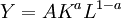
This is a Cobb-Douglas function where Y represents the total production in an economy. A represents multifactor productivity (often generalized as technology), K is capital and L is labor.

An important relation in the macro-production function:

$Y=AK^aL^{1-a}\ \leftrightarrow y=Ak^a$

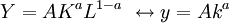
Which is the macro-production function divided by L to give total production per capita y and the capital intensity k

[edit] GDP equation

$Y=C+G+I+NX\,$

Where C is private consumption, G is public consumption, NX is net exports, and I represents investments, or savings. Note that in the Solow model, we represent public consumption and private consumption simply as total consumption from both the public and government sector. Also notice that net exports and government spending are excluded from Solow's model. This equation is called the GDP equation because it is calculated much the same way as is the Gross domestic product (or more precisely the Gross national product).

[edit] Savings function

$I=sY\,$

This function depicts savings, I as a portion s of the total production Y.

[edit] Change in capital

$\Delta K=sY-\,$ $\delta K\,$

The $\delta\,$ is the rate of depreciation.

[edit] Change in workforce

$L_{t+1}=L_t(1+gL)\,$

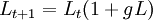
gL is the growth function for L.

[edit] The model's solution

First we'll need to define some growth functions.

1. Growth in capital $gK=\frac{\Delta K}{K}$

2. Growth in the GDP 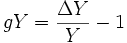$gY=\frac{\Delta Y}{Y}-1$

3. Growth function for capital intensity 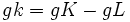$gk=gK-gL\,$

[edit] Solution assuming no multifactor productivity growth

This simplification makes the solution's derivation more comprehensible, as it allows the following calculations:

$gK=\frac{\Delta K}{K}\rightarrow\frac{sY-dK}{K}\rightarrow\frac{sY}{K}-d$

When there is no growth in A then we can assume the following based on the first calculation:

$gK=gL=gY\,$

Moving on:

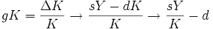
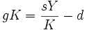$gK=\frac{sY}{K}-d$ Divide the fraction by L and you will see that $gK=\frac{sy}{k}-d$

$gK=\frac{sy}{k}-d\rightarrow\frac{sAk^a}{k}-d\rightarrow\frac{sA}{k^{1-a}}-d$

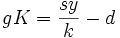
By subtracting gL from gK we end up with:

$gk=\frac{sA}{k^{1-a}}-(d+gL)$

If k is known in the year t then this formula can be used to calculate k in any given year.

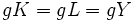
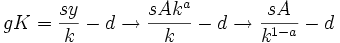
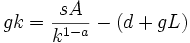
In the first segment on the right side of the equation we see that $\lim_{k \to 0} gk=\infty$ and $\lim_{k \to \infty}gk=-(d+gL)$

Deriving the Steady-state equation:

$d (K / L) / d t = d (k) / d t$ where $k = K / L$ and k denotes cper worker.

Differentiating we obtain:

$dk/dt=(\frac{dK L-dL K}{L^2})/dt$ \frac{}{} which is

$dk/dt=(dK/L)/dt-(\frac{dL}{L}\frac{K}{L})/dt)$ we know that

$(d L / L) / d t$ is the population growth rate over time denoted by n.

Furthermore we know that

$d K / d t = s Y - x K$

where x is the depreciation rate of capital.

Hence we obtain:

dk=sy-(n+x)k

which is the fundamental Solow equation. The same can be done if technological progress is included.

[edit] A Simple Explanation

Consider a simple case Cobb-Douglas production function:

$Y=K^{\alpha}N^{1-\alpha}\,$ ,

where $Y$ is level output, $K$ level of capital, $N$ level of employment (given, fixed), and $0 < α < 1$ is relative capital intensity (given, fixed). Net capital accumulation per capita in period $t$ is given by:

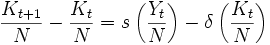$\frac{K_{t+1}}{N}-\frac{K_t}{N}=s\left(\frac{Y_t}{N}\right)-{\delta}\left(\frac{K_t}{N}\right)$ ,

where $s$ is the savings rate, and $δ$ the depreciation rate. The economy reaches a steady state level of output and capital when net capital accumulation per capita is zero. That is,

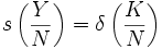$s\left(\frac{Y}{N}\right)={\delta}\left(\frac{K}{N}\right)$ ,

the amount of total investment (left side) is equal to the amount of capital depreciation (right side) in any given period. From the production function we know that output per capita is given by:

$\frac{Y}{N}=\left(\frac{K}{N}\right)^\alpha$ ,

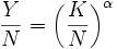which implies that the steady state levels of capital and output, denoted by asterisks, are:

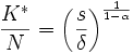$\frac{K^*}{N}=\left(\frac{s}{\delta}\right)^{\frac{1}{1-\alpha}}$ ,

and

$\frac{Y^*}{N}=\left(\frac{s}{\delta}\right)^{\frac{\alpha}{1-\alpha}}$ .

for given values of $s$ , $δ$ , and $α$ .

Now consider output as a Cobb-Douglas function of capital and effective labor $A N$ :

$Y=K^{\alpha}\left(AN\right)^{1-\alpha}\,$ ,

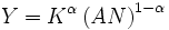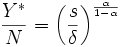
where increases in technology $A$ positively affect output $Y$ by improving the efficiency of labor $N$ . If technology grows at a constant positive rate of $g A$ , and labor at $g A$ , then their product $A N$ grows at a rate approximately equal to $g A + g N$ . Consequently, the steady state level of output per unit of effective labor (derived from the original steady state condition)

$\frac{Y^*}{AN}=\left(\frac{s}{\delta}\right)^{\frac{\alpha}{1-\alpha}}\,$

is actually declining since output $Y$ is by definition growing at zero in the steady state (left side numerator), whereas (in the denominator) effective labor is growing at $g A + g N > 0$ . Therefore, in order to offset this additional source of per unit erosion in steady state output, the steady state condition must be modified to read:

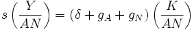
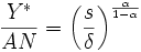
$s\left(\frac{Y}{AN}\right)=\left(\delta+g_A+g_N\right)\left(\frac{K}{AN}\right)$

total investment (left side) must equal the amount of growth in effective labor in addition to the amount of capital depreciation. This modification implies that the steady state level of output per unit of effective labor is

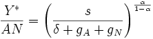$\frac{Y^*}{AN}=\left(\frac{s}{\delta+g_A+g_N}\right)^\frac{\alpha}{1-\alpha}$ .

Similarly, the steady state level of capital per unit of effecitve labor is

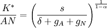$\frac{K^*}{AN}=\left(\frac{s}{\delta+g_A+g_N}\right)^\frac{1}{1-\alpha}$ .

Note: Although per unit growth is zero, the absolute levels of output $Y *$ and capital $K *$ in the steady state are still growing at a constant positive rate $g A + g N > 0$ . This result is sometimes referred to as balanced growth. Also note that the savings rate $s$ does not affect the rate of growth in the steady state, although it does still contribute to the initial level of output and capital at the start of a period of balanced growth.

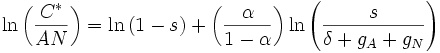
The golden rule savings rate $s *$ maximizes the steady state level of aggregate consumption $C *$ per unit of effective labor, as defined by the national income (GDP) identity:

$\frac{Y^*}{AN}=\frac{C^*}{AN}+\frac{I^*}{AN}$ .

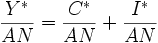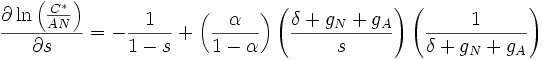
Assuming that the steady state level of investment $I *$ equals $s Y *$ , the golden rule savings rate solves the unconstrained maximization problem

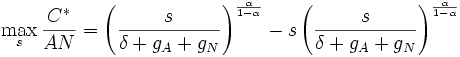$\max_s \frac{C^*}{AN}=\left(\frac{s}{\delta+g_A+g_N}\right)^\frac{\alpha}{1-\alpha}-s\left(\frac{s}{\delta+g_A+g_N}\right)^\frac{\alpha}{1-\alpha}$ .

Since

$\ln{\left(\frac{C^*}{AN}\right)}=\ln{\left(1-s\right)}+\left(\frac{\alpha}{1-\alpha}\right)\ln{\left(\frac{s}{\delta+g_A+g_N}\right)}$ ,

this implies

$\frac{\partial\ln{\left(\frac{C^*}{AN}\right)}}{\partial s}=-\frac{1}{1-s}+\left(\frac{\alpha}{1-\alpha}\right)\left(\frac{\delta+g_N+g_A}{s}\right)\left(\frac{1}{\delta+g_N+g_A}\right)$ ,

setting equal to zero and simplifying,

$0=-s+(1-s)\left(\frac{\alpha}{1-\alpha}\right)$ ,

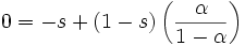finally,

$s^*=\alpha\,$ .

Note: This implies that aggregate consumption per unit of effective labor in the steady state is maximized when the savings rate is exactly equal to the relative intensity of capital in the production function.

[edit] See also

[edit] External links

Java applet where you can experiment with parameters and learn about Solow model

[edit] Notes

^ Solow. R. M. (1957), Technical Change and the Aggregate Production Function. Review of Economics and Statistics, 39.

Retrieved from "http://en.wikipedia.org/wiki/Exogenous_growth_model"

Categories: Macroeconomics | Economic growth